How I Make Weekly Price Estimates

Bayesian Linear Regression experimentation

The other day, I wrote about a common misuse of statistics and how I adapted my behaviors regarding probabilities.

[Crypto] Analysts Have a Stats Problem

I’m pretty sure most technical analysts who release products or voice their opinions have included price ranges, their best guess of where asset prices will fluctuate over a specified amount of time. Even I have provided that in my history of publications. It’s helpful to have an idea ahead of time to manage expectations.

When I created price ranges, there wasn’t a defined structure, mostly gleaned from subjective opinions and intuition. I’d look at current trading ranges containing price action and one beyond that to create some logical expectation.

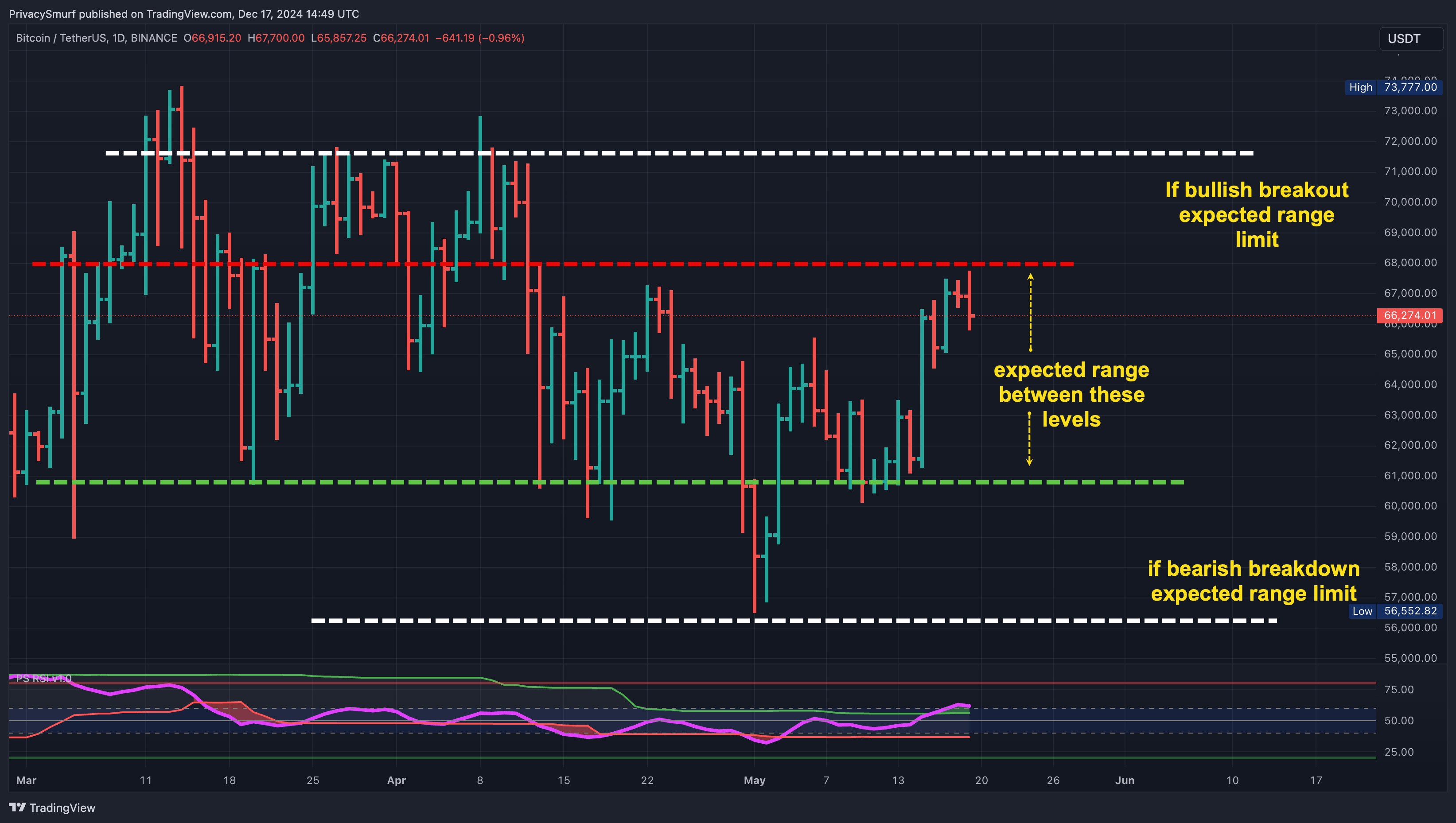
This is a perfectly acceptable approach, but it’s very subjective. Accuracy stems from a healthy portion of luck and interpretations of market technicals such as momentum, volume, and historical knowledge. Others can’t precisely replicate this, and other analysts will create interpretations differently. I didn’t necessarily change so others could duplicate me, but I wanted to incorporate more objective and probabilistic techniques.

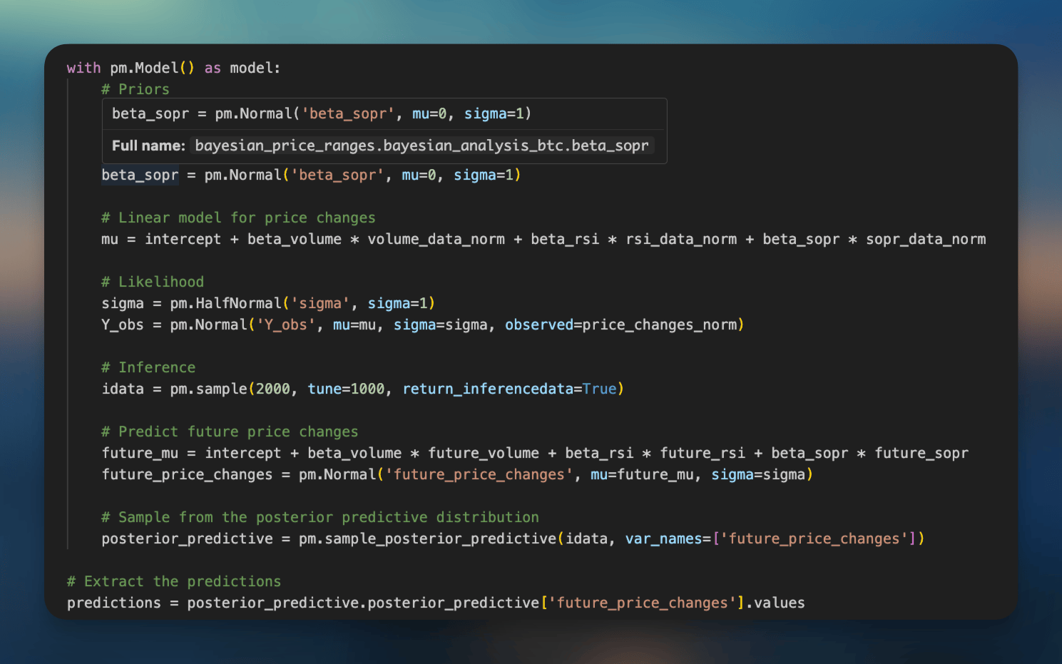
Enter Bayes Theorem and Linear Regression. I said this section of posts would be dense, but don’t worry; I won’t go into deep maths and give you a single-sentence summary.

Bayesian Linear Regression is a statistical method that models the relationship between variables while incorporating prior beliefs and uncertainty into the estimates using Bayes’ Theorem.

What does that mean for my implementation?

First, I’m grabbing intraday (2HR timeframe) values for closing prices, volume, the cyclic RSI, and the SOPR (an on-chain metric).

Then, I process the historical data through a Python package dedicated to statistical modeling, PyMC. I’m essentially using the history of the metrics above as prior knowledge, trying to determine how they interact to create a possible future, given what metrics look like now.

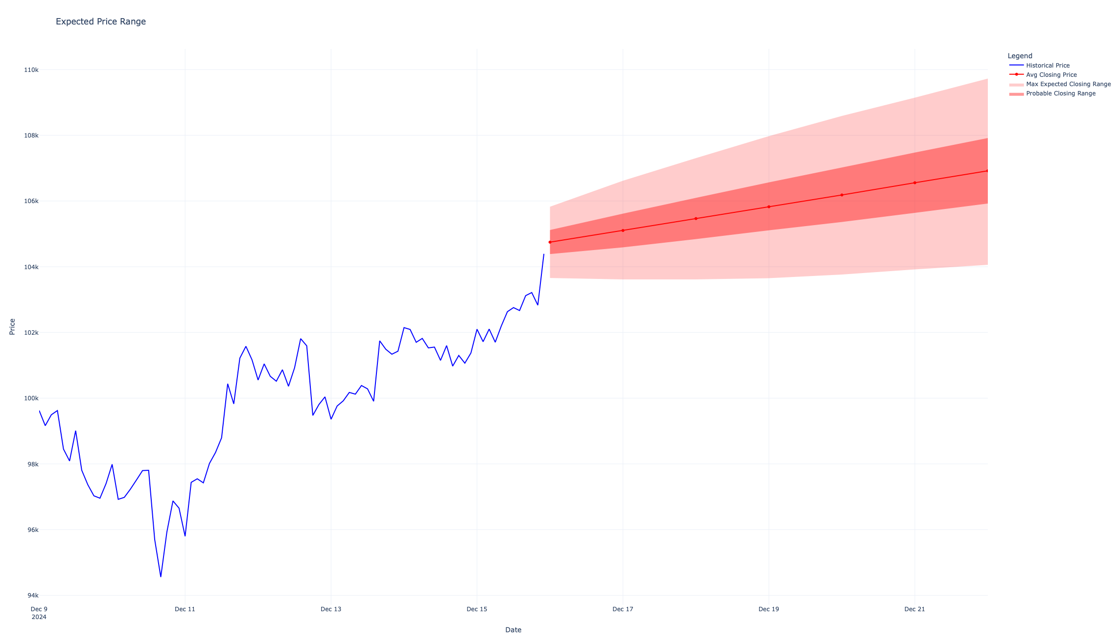
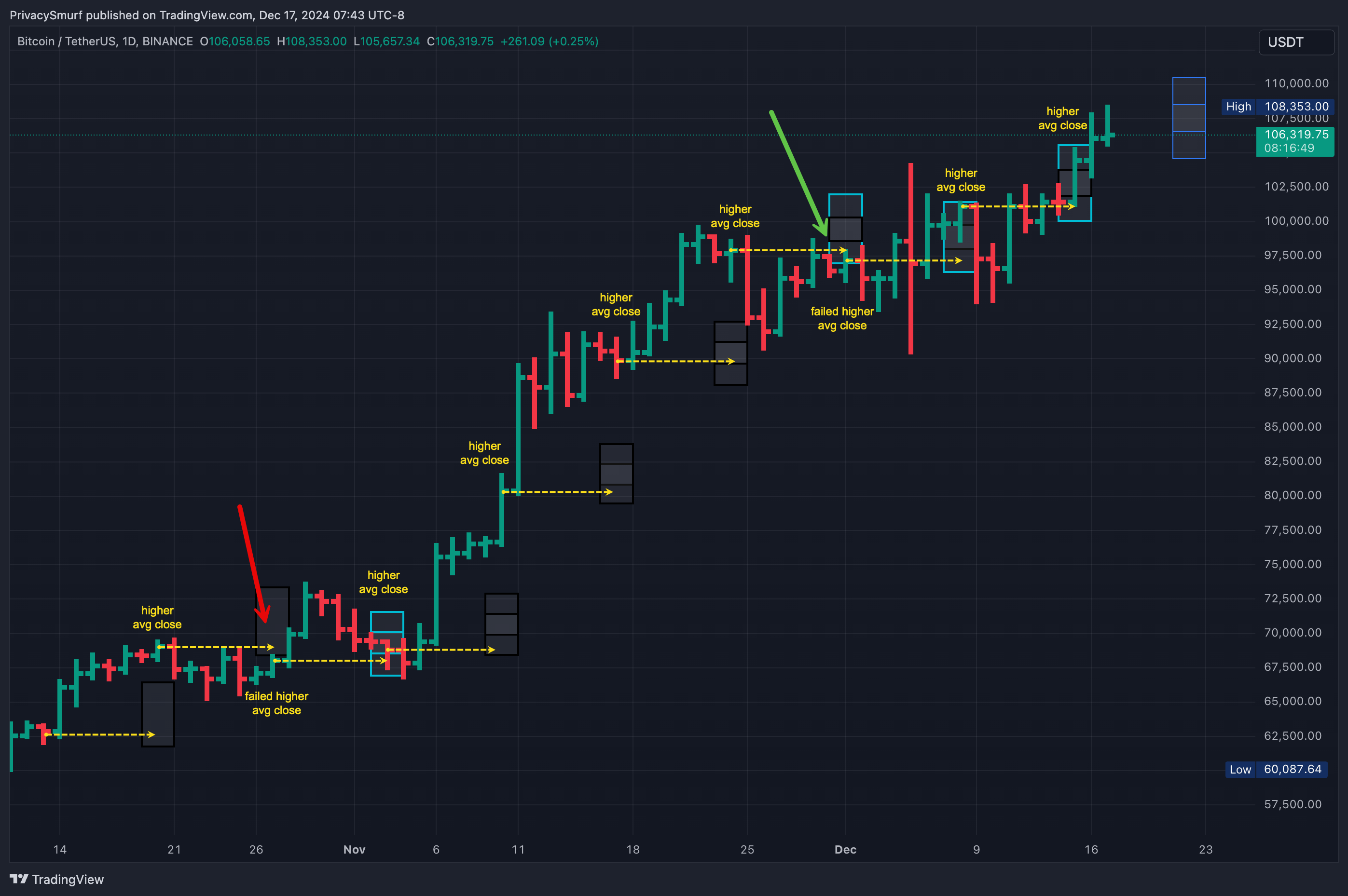
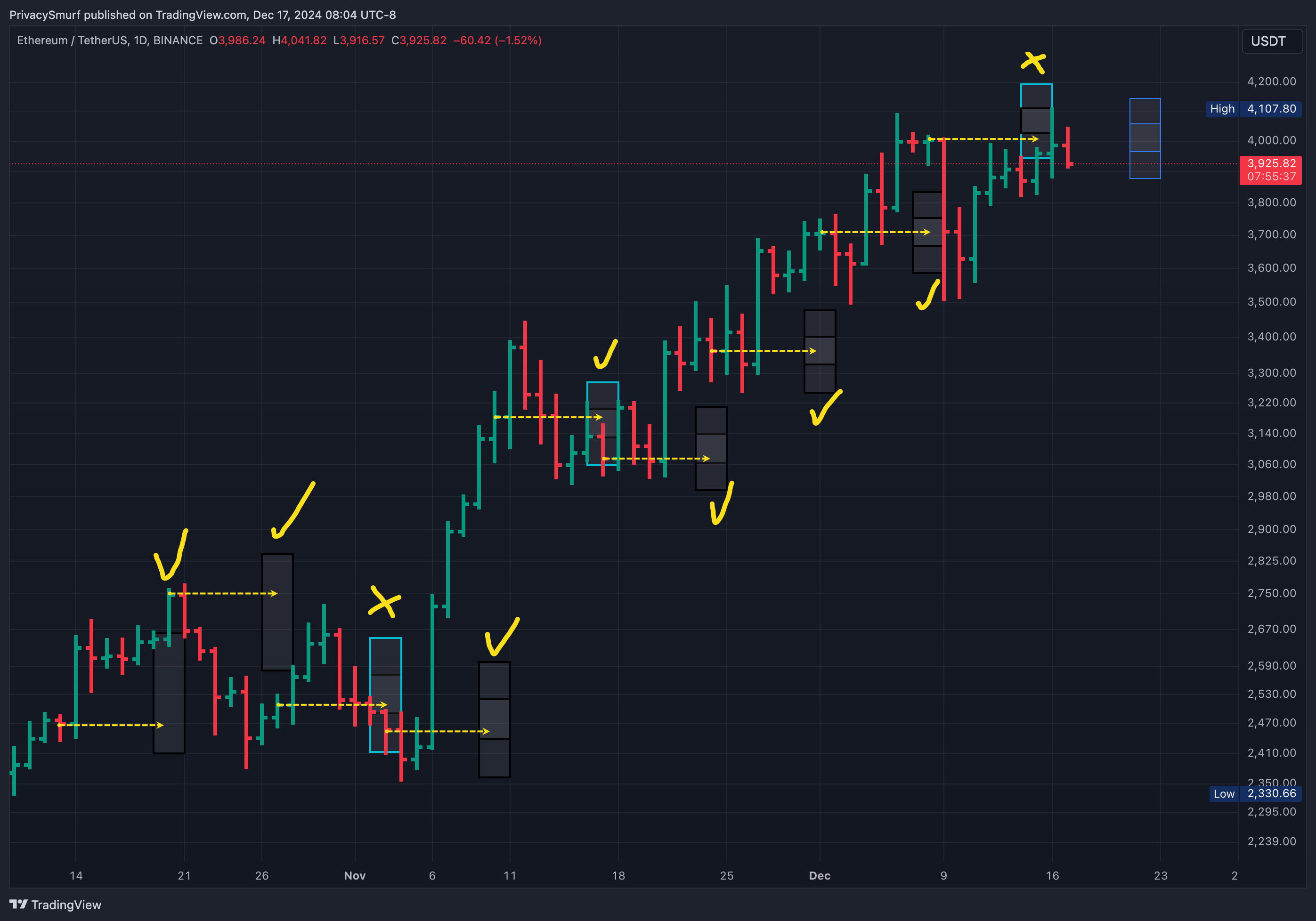
After that process is complete, I plot the results. This is what I include in the weekly updates. The blue line is closing prices for the past week on the 2HR timeframe. The light red shaded area is the range for closing prices daily at a 95% probability. The dark red shaded area is the range for closing prices daily at a 50% probability. The dark red line in the middle shows the average expected closing price. I’m less concerned about the day-to-day closing prices and more interested in the final one at the week's close.

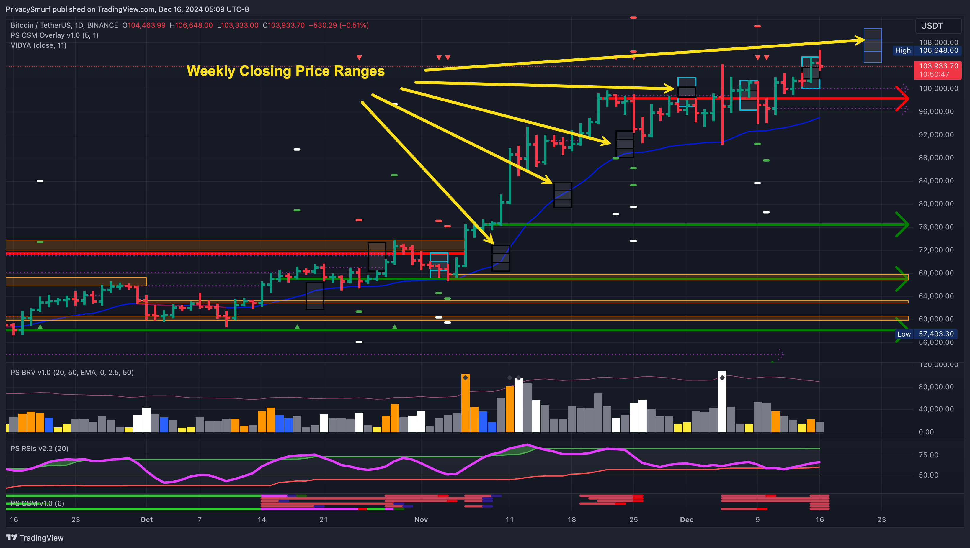
In my updates, I present the range for the weekly closes on the price chart in this way: Black borders indicate missed ranges and light blue borders indicate accurate predictions. You can also see the plotted difference between the 50% and 95% ranges.

This would be expressed purely scientifically: “Given the current technicals, I can say with 95% confidence that the closing price for BTC this week will be between $104058.60 and $109726.06.”

This is all a new venture for me, and I’m not exactly sure what to do with it yet regarding viewing it as an analytical tool or actionable resource. I’ve still got some coding to build out the means to backtest the accuracy, and right now, I’m just forward testing.

---

Some initial observations:

It’s pegging the week’s direction on BTC quite accurately. Let’s take the closing price from the week of the update and compare that to the forecasted average closing price. The weeks have closed in line with the directionality of the predicted average. When the forecasted average was above the weekly close, the week closed bullish, failing only twice: once in week two and again in week seven. However, week seven still closed inside the expected ranges.

It’s less accurate on ETH overall, with one less precise range prediction but similar directionality estimations, two incorrect. However, both inaccurate mean directions were still close to the maximum expected range, so I guess it’s a wash.

We haven’t yet experienced any real-time trend changes, so I’m not sure how accurate this process will be. I’m not measuring any mean reversion metrics; however, I may add something like that. I’m also considering adding a secondary volume metric.

So far, this has been an enjoyable experience. I typically create my expectations based on TA and intuition, then run the data and evaluate its output. I don’t know if I’ll ever get to a place where I stop my manual process, but who knows? Ultimately, I think the less I have to rely on my guesses, the better. At least I’ll have some quantifiable risk (sort of, but that’s a topic for another day).

I’m open to any suggestions in this process. There’s no bad idea. Drop them in the comments. Thanks.

@ThePrivacySmurf